You have likely read about how the field of machine learning (ML) is making serious inroads into how Wall Street is operating, with firms like BlackRock, Bridgewater, D. E Shaw & Co. among many others all actively using ML and hiring experts in that field.
The team at Deep Value has been using ML for the past few years and has prepared some research aimed at desks new to field — in this installment, on using machine learning to combine trading alphas.
- Off-the-shelf machine learning, and especially support vector machines, are a defensible starting point for automatedly combining alphas, over purely linear and simple regression-based approaches.
- Other (clustering and boosting) approaches also show promise, while needing work and calibration to deal with respectively high dimensionality, and high noise.
- ML-based approaches come with opacity, and the ability of ML models to evolve with the markets can hamper an understanding of what they are doing.
The link to the research is here.
Disclaimers apply.
July 25 2017 · Filed in: research
What is Parity at the NYSE and Why Should You Care?
The NYSE is the only exchange offering “parity allocation” of all trades. Roughly 600 million shares trade each day at the NYSE in the regular session; virtually all these trades happen at the NYSE matching engine via that parity allocation model that enables orders from multiple Floor brokers, DMMs and DOT orders at the top of the book to share executions at the same price point.
Floor broker orders, posted to the NYSE via what are called e-Quotes, can in particular yield higher fill rates and lower adverse selection owing to this parity model.
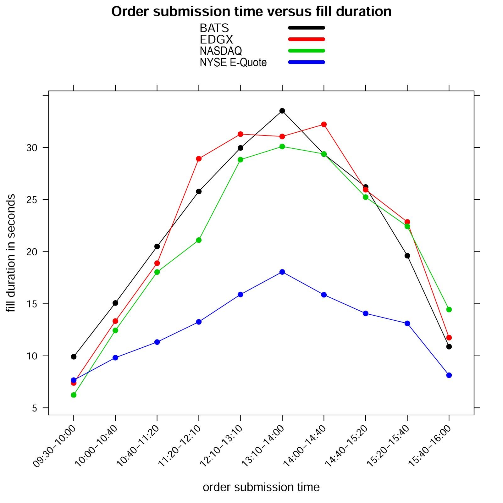
Here, for example, is an analysis of production data from the period Nov 2014-Feb 2017, examining a total of roughly a 100 thousand randomly picked orders across the 4 examined destinations (details available on request). Compare e-Quotes’ fill times with that of orders placed at other marketplaces.
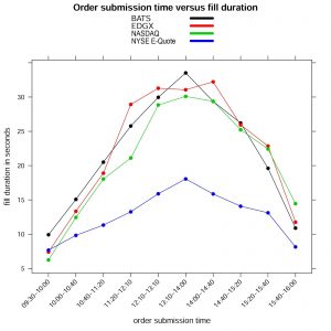
Fig 1: Time to fill is lower via (Floorbroker sent) eQuotes
Introducing Deep Value’s FAST Parity Service: A Game Changer
Deep Value is now offering, via its Floor Access Strategies (FAST) Parity Service, the first Floor-wide access to parity for buy-side firms that wish to use custom algo strategies.
Currently, custom strategies (as opposed to benchmark strategies) that receive parity allocations are used only by a limited base of trading customers who have contracted with NYSE-approved TPA providers.
The Deep Value Floor FAST Parity Service aims to broaden that base, while conforming to the requirements on NYSE TPA providers. Deep Value is offering this in partnership with Floor brokers, and the service is available for customers of any Floor broker to use. It will allow trading firms that were previously deterred from bearing TPA costs — costs of the trading stacks that run their own custom trading logics, separate market data infrastructure and associated hosting and connectivity — to now access parity more easily, and from their pre-existing trading infrastructures.
Thus Deep Value’s FAST Parity service allows Floor brokers to present their traditional e-Quote as a low-latency DMA endpoint that is simply accessed via FIX from customers’ existing servers.
When Posting at Parity Typically Outperforms
While the usual disclaimers apply, in our research we observe that the value of parity via the e-Quote is most pronounced when book depth across marketplaces is relatively high (at least several hundred shares shown), when spreads are not too wide, and as in Fig 1, away from the open and close.
April 13 2017 · Filed in: research
The newly introduced Deep Value Floor Close route allows participation in the NYSE closing auction nearly a full fifteen minutes after the usual 3:45 p.m. deadline to participate in the close (subject to limitations and disclaimers, driven by market quality, compliance and other considerations). The upshot is that a straightforward trading strategy that in one case simply offsets the imbalance, and in another case uses a factor model in addition to the imbalance signal, yields decent Sharpes in the datasets examined.
Barebones Trading Strategy Based on the Imbalance Signal Alone
This analysis was done using the NYSE-listed names in S&P 500. The date range for the analysis is Nov 2013 – April 2015.
We use the imbalance feed, and trade on the same side of imbalance at 3:45. The trading footwork is kept minimalist to evidence that there is no (or at least little room for) “data mining” — so the strategy hasn’t been carefully constructed to show profitability on the specific stocks and date ranges backtested. So we don’t do marginal risk calculations or even factor neutralize. The strategy is “one shot” in that it doesn’t adapt when imbalance quantities change. We trade only the NYSE-listed subset of the S&P 500 names, instead of using the entire (sufficiently liquid) universe of NYSE-listed names and so, on. But as you will see, even this starting point shows promise.
For each name that we choose to enter into, the size we wish to trade into is chosen to be 10 basis points of the 20 day Average Daily Volume (ADV) traded in that name. The actual entry trading logic backtested uses only displayed orders, places those at the NBBO on the same side (so on the national best ask if selling), at the NYSE alone and pegs to the same side.
We exit all positions by participating in the close via market orders.
Comments on Simulation Fidelity
Our market models implement the market-specific fill logic by tracking the position of our simulated order in the order book. As prints lift off lots of our orders advance. If the market trades through our price we give ourselves a fill. And so on, with some care.
In the interest of having high fidelity in our simulations, we take certain steps. Our market models do not account for the incremental market impact of displayed sizes, and also do not simulate the incremental impact from the executions received in the backtesting. We address these sources of simulation errors by choosing display sizes that are small relative to the sizes already on the book at order placement time, and by keeping the liquidity demanded low relative to the rate at which the market prints.
While these steps result in simulations that track real-world production outcomes well, with this conservatism fill rates that are achieved are lower. To address this, in the trading simulation, we peg to the inside market, making our limits more aggressive with the market when the market moves away. We inject latency into the simulation in the order of several 10s of milliseconds so there is no presumption of needing high quality trading and market data infrastructure, and of having low latency trading fabrics to make this chasing work.
Order sizes resulting are small enough that the displacement to the closing auction price when we participate at the close is negligible. In the simulations we track order book depth at order placement time, track prints and cancellations, use realistic mil rates and fees, and keep quoted sizes down. Simulations track actual trading outcomes and production fill quantities well. In our market model for the NYSE, we use a price-time priority fill model.
Transaction Cost Assumptions
We state explicit transaction costs and rebates in mils (cents per 100 shares). We assume that NYSE entry fills generate a rebate of 15 mils (this is indeed the prevalent rebating regime for liquidity contributed via DOT). Exit fills, fills that executed at the closing auction, are priced to cost 3 mils at the Exchange, and that in addition, there is a clearing and DMA fee that has also been accounted for.
Outcomes From Using the Imbalance Feed Alone
With the preliminaries done, let us look at results. Outcomes are shown in Table A, under the column “Imbalance Signal Alone“: Note that using the imbalance feed alone, and not using the factor model in addition, generates a Sharpe of a little over 1. Note that in some names we don’t get filled by the market in the entry trade, and hence we wind up trading on average only 295 names each day from (NYSE-listed subset of) the S&P 500.
Combining the Imbalance Feed with a Factor Model
We next add in a fundamental factor model intraday to generate buy and sell signals. We construct normalized factors using stock-specific fundamental data such as earnings yield, growth, beta, etc. The direction (long or short) is decided based on the sign of the idiosyncratic return (actual – estimated price) at 3:45. If the idiosyncratic return is positive, the stock is over-valued and we expect the price to drop going towards close. Positions are taken post 3:45 based on the premise that there is factor reversion. We require both the imbalance feed signal and the factor model’s reversion signal coincide prior to trading. As before we exit our positions at the closing auction, after being in the market for roughly 15 minutes.
Table A under the column headed “Factor Model Residue Reversion + Imbalance Signal” shows metrics when we combine the imbalance signal with that from the factor model. Note that the Sharpe and other PnL metrics have improved — the Sharpe is now 1.5, drawdowns are less severe compared to the average daily productivity and so on.
[table id=1 /]
Data: NYSE-listed names in S&P 500. The date range for the analysis is Nov 2013 – April 2015
Conclusion
We have shown that getting extra 15 minutes to trade at the close is valuable in a particular trade where we offset the imbalance, and use the Floor Close route to flatten. There are, of course, many more reasons why it might be better to trade at the close at 3:59:49 instead of at 3:45 — every high frequency strategy, every market making strategy, in fact pretty much every strategy that looks to be flat at end of day could use a route that trades later in the day. Contact us or your Floor Broker if you would like to explore whether this route can be of help to you.
Figure A: Equity lines for cumulative portfolio return: with transaction costs. The plot depicts the performance of the imbalance signal, factor reversion strategy and the combined strategy.

January 4 2017 · Filed in: research